Machining or metal cutting is one important aspect of the production system. Ultimate objecting of machining is to give intended shape, size and finish by gradually removing material from workpiece. Relevant steps such as removal of material, setting the job and cutting tool, and dispatching the machined job consume substantial amount of time, which are at least not negligible. For effective planning of the entire production, overall machining or cutting time must be incorporated.
Now-a-days the primary goal of industries is to manufacture the product at a faster rate but at minimal cost and that too without sacrificing product quality. As long as conventional machining is utilized, in order to fulfill first requirement (faster production rate), the cutting speed and feed rate should have to be increased. However, this may lead to reduced cutting tool life due to faster wear rate and higher heat generation. Hence, cutting tool is required to change frequently, which will ultimately impose a loss for the industry as a result of idle time for changing tools. Cost of tool is also not negligible. Therefore abrupt increase of cutting speed and feed rate is not a feasible solution; rather, an optimization is necessary.
Expressing total production cost in terms of time elements
In machining economics, cost elements are derived from time by multiplying with a conversion factor. Basically overall or total machining time (Tm) is the summation of three different time elements closely associated with the machining or metal cutting process. These three elements include—actual cutting time (Tc), total tool changing time (Tct) and other handling or idle time (Ti). Mathematically, Total Time for Machining (Tm) can be expressed as:
Tm = Tc + Tct + Ti
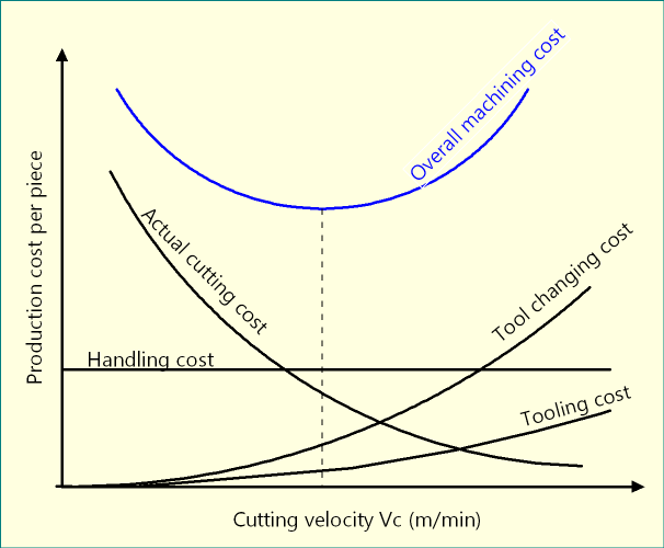
Apart from these three time elements and associated cost, cost of the cutting tool is also another factor to consider for any optimization. All these time or cost elements, except handling time, are affected by the variation of cutting speed and feed rate as depicted below.
If K1 be the cost-time conversion factor for machining and K2 be the cost-time conversion factor for tool sharpening or price of new tool, then overall machining cost per piece (Cp) can be expressed as follows. For better understanding of these individual time or cost element, you may read: Economics of machining – cutting time, tool changing time & idle time.
Cp = (Actual cutting cost/piece) + (Tool changing cost/piece) + (Handling cost/piece) + (Tooling cost/piece)
Cp = K1 {(Actual cutting time/piece) + (Tool changing time/piece) + (Handling time/piece)} + K2 {(Tooling cost/piece)}
Cp = K1 {Tc + Tct + Ti} + \(\left( {{{{T_c}} \over {TL}}} \right) \times {K_2}\)
Expressing production cost in terms of cutting velocity
If, Lc is the total length of cut (mm), N is the spindle speed (rpm) and s is the feed rate (mm/rev), then estimated machining time can be expressed as:
Actual Cutting Time (Tc) = \({{{L_c}} \over {N.s}}\)
In most of the cases, where either workpiece or cutting tool is rotating, the spindle speed (N) and cutting velocity (Vc) are interchangeable. However, cutting velocity also depends on the diameter of the job/cutter (D). Cutting velocity can be expressed, in terms of speed and diameter of job or cutter (whichever is rotating), as follows. For better understanding of this conversion, you may read: Cutting speed and cutting velocity in machining.
Cutting velocity (Vc) = \({{\pi DN} \over {1000}}\)
Now, \({T_c} = {L \over {N.s}}\)
or, \({T_c} = {L \over {\left( {{{1000{V_C}} \over {\pi D}}} \right)S}}\)
or, \({T_c} = {{\pi DL} \over {1000{V_C}}}\)
Again from Taylor’s Tool Life Formula, we know:
\({V_c}{(TL)^n} = C\)
So, \(TL = {\left( {{C \over {{V_c}}}} \right)^n}\)
Substituting these values, we get production cost per piece:
\({C_p} = \left\{ {{{\pi DL} \over {1000{V_c}s}}{K_1}} \right\} + \left\{ {{T_i}{K_1}} \right\} + \left\{ {TCT{{\pi DL} \over {1000{V_c}s}}{{\left( {{{{V_c}} \over C}} \right)}^{1/n}}{K_1}} \right\} + \left\{ {{{\pi DL} \over {1000{V_c}s}}{{\left( {{{{V_c}} \over C}} \right)}^{1/n}}{K_2}} \right\}\)
Derivation for optimum cutting velocity for minimum production cost
There exists another similar optimization model where the objective is to maximizing production rate, instead of minimizing production cost. You may read that model here: Optimum velocity & tool life for maximum production rate in machining. Now let up optimize cutting velocity for minimum production cost. This economic model is also known as Gilbert’s Model (1952). From the above equation, production cost can be expressed as:
\({C_p} = \left\{ {{{\pi DL} \over {1000{V_c}s}}{K_1}} \right\} + \left\{ {{T_i}{K_1}} \right\} + \left\{ {TCT{{\pi DL} \over {1000s}}{{\left( {{1 \over C}} \right)}^{1/n}}{{\left( {{V_c}} \right)}^{{{1 – n} \over n}}}{K_1}} \right\} + \left\{ {{{\pi DL} \over {1000s}}{{\left( {{1 \over C}} \right)}^{1/n}}{{\left( {{V_c}} \right)}^{{{1 – n} \over n}}}{K_2}} \right\}\)
Assuming cutting velocity as the only independent variable, let us differentiate cost per piece with respect to cutting velocity:
\({{d{C_p}} \over {d{V_c}}} = \left\{ {{{\pi DL} \over {1000s}}{K_1}\left( { – {V_c}^{ – 2}} \right)} \right\} + 0 + \left( {{K_1}TCT + {K_2}} \right)\left( {{{\pi DL} \over {1000 \times s \times {C^{1/n}}}}} \right)\left( {{{1 – n} \over n}} \right){\left( {{V_c}} \right)^{{{1 – 2n} \over n}}}\)
Now for minimum production cost, \({{d{C_p}} \over {d{V_c}}} = 0\)
Therefore,
\(\left\{ {{{\pi DL} \over {1000s}}{K_1}} \right\}{1 \over {{V_c}^2}} = \left( {{K_1}TCT + {K_2}} \right) \times \left( {{{\pi DL} \over {1000 \times s \times {C^{1/n}}}}} \right)\left( {{{1 – n} \over n}} \right){\left( {{V_c}} \right)^{{{1 – 2n} \over n}}}\)
\(\left( {{n \over {1 – n}}} \right)\left( {{{{K_1}} \over {{K_1}TCT + {K_2}}}} \right){C^{1/n}} = {\left( {{V_c}} \right)^{{{1 – 2n} \over n} + 2}}\)
\({\left( {{V_c}} \right)^{1/n}} = \left( {{n \over {1 – n}}} \right)\left( {{{{K_1}} \over {{K_1}TCT + {K_2}}}} \right){C^{1/n}}\)
\({V_c} = C{\left\{ {\left( {{n \over {1 – n}}} \right)\left( {{{{K_1}} \over {{K_1}TCT + {K_2}}}} \right)} \right\}^n}\)
Hence optimum cutting velocity for minimum production cost be:
$${V_{c,optimum}} = C{\left\{ {\left( {{n \over {1 – n}}} \right)\left( {{{{K_1}} \over {{K_1}TCT + {K_2}}}} \right)} \right\}^n}$$
Derivation for optimum tool life for minimum production cost
Let us apply Taylor’s Tool Life Equation in order to calculate optimum tool life for minimum production cost using the optimum cutting velocity. So,
Taylor’s Tool Life Formula: \({V_c}{(TL)^n} = C\)
Since, \(TL = {\left( {{C \over {{V_c}}}} \right)^{1/n}}\)
or, \(TL = \left( {{{1 – n} \over n}} \right)\left( {{{{K_1}TCT + {K_2}} \over {{K_1}}}} \right) \)
Hence optimum tool life be:
$$T{L_{optimum}} = \left( {{1 \over n} – 1} \right)\left( {{{{K_1}TCT + {K_2}} \over {{K_1}}}} \right)$$
Final formulas
$${V_{c,opt}} = C{\left\{ {\left( {{n \over {1 – n}}} \right)\left( {{{{K_1}} \over {{K_1}TCT + {K_2}}}} \right)} \right\}^n}$$
$$T{L_{opt}} = \left( {{1 \over n} – 1} \right)\left( {{{{K_1}TCT + {K_2}} \over {{K_1}}}} \right)$$
Reference
- Book: Metal Cutting: Theory And Practice by A. Bhattacharya (New Central Book Agency).
- Book: Machining and Machine Tools by A. B. Chattopadhyay (Wiley).